Random number generators based on transistor noise are being used for many years. To ensure the numbers are uniformly distributed, this project uses an integrated chi-square test to check the output and automatically restart the generator if the test fails. This makes the difference, compared to other projects.

Concept
You are familiar with the fact, that computers can only generate pseudo random numbers. Today you can get quite good uniformly distributed numbers, but they are never perfect. To get perfect random numbers, you may pick the amplitude value of a white noise signal at an arbitrary time.

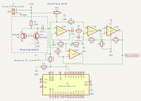
The Analog Circuit [1]

The white noise signal is available at the output „noise_analog." You can feed it into an amplifier and, using your spectrum analyzer, check whether the signal exhibits amplitude loss over the amplifier's bandwidth. [2] [3]

The heart of the circuit is a noise signal source built with transistors Q1 and Q2. Essentially, almost any NPN transistor can be used here. A good choice is the BC548C. The 2N2222 is also well-suited.

If we had wanted to use and amplify the transistors' inherent noise, this project would have been barely feasible. As yo can see in the schematic, transistor Q1 is connected "backwards." At breakdown voltage, the emitter-base junction of Q1 begins to conduct while producing significant noise. Q2 does not contribute to this; it serves as a current source.

The breakdown voltage depends on multiple factors. In any case, it is above 5 V, so we use 15 V (which is generated by a step-up converter MT3608).

The subsequent operational amplifiers U1B, U1C, and U1D function as a buffer (U1B) and amplifiers. U1C is biased at the non-inverting input with a voltage through the trim pot RV1. This influences both  gain and the operating point. We need to ensure that the operational amplifier — capable of delivering up to 15 V rail-to-rail — only outputs the amplified noise signal, which must not exceed 3 V, as the nano V3's analog input A0 will not tolerate higher voltages.

We first build and calibrate the noise generator. When this part is running perfect and the output voltage is correct, you may connect the nano V3 microprocessor.

As we receive a C-coupled signal (from C1) at pin 5 of the TL074, which fluctuates around the zero point, U1A adds approximately ½ of the 15V (i.e., about 7.5 V) through a 1MΩ resistor (R5). This shifts the zero line from -7.5 V to 0 V. The noise signal now fluctuates between 0 V and the respective maximum amplitude. This approach eliminates the need for a negative power supply.

The circuit requires your attention at several points. For one, there is quite a bit of variation in the characteristics of npn-transistors. I’ve built several versions of the circuit. In one version, I only needed U1D as a buffer and not as an amplifier because the 2N2222 transistors produced 250 mV of noise. In this case, R8 is replaced with a wire bridge and R9 is omitted compleately. Unfortunately, you can only test this by trial and error and check it on the oscilloscope.

Moreover, adjusting RV1 is a bit critical. The potentiometer is initially turned all the way to the ground side. It’s best to measure the voltage at the pot’s wiper, 0 volts on start. Then power up and slowly turn the 10-turn pot until you obtain a clean noise signal with an amplitude of about 2.5 V. Please take a look at the video as reference for you [2].

The video demonstrates that the signal "dances" above the zero line as espected. However, there is a small DC offset (abt 0.25 V DC) between the lower mark on the oscilloscope and the smallest amplitude of the noise signal, which we will later "subtract" using the sketch.

Typically, RV1 is set so that the bias voltage is ≤ 0.3 V. Please ensure that the output amplitude of the noise signal remains below 3 V.

One note about the circuit layout: The MT3608 step-up converter generates minimal noise, but due to the high gain and sensitivity of the circuit, the converter’s 150 kHz signal can couple into the system, causing systematic errors and compromising the randomness. If you position the converter next to the nano V3 as shown in the photos of the prototype, I didn’t notice any issues [5].

The Sketch .
The sketch is split up into six .ino files for better readability and understanding. Please don’t mind that some filenames are in German. The project was originally made for domestic users, but as there was so much positive feedback, I decided to translate (most of) the sketches.

Command Processor <MD_cmdProcessor.h>
For most of my lab projects I use MD_cmdProcessor.h. It helps a lot to make the communication between your PC and the MCU simple and structured. You can find MD_cmdProcessor.h on GitHub easily and it’s easy to use. You may add a Bluetooth module and control your project by your mobile phone easyly.

Everything is built around the MD_cmdProcessor.: All handlers are placed at the top of the sketch. The command-definition table follows, then the handlerHelp.

As soon as you are at this point, most of the sketch is finished. The rest is quite simple:

Let’s go through the sketch. We have some variable definitions at the top. We define an array of 300 for the random numbers. 300 numbers is the maximum with the nano V3; the compiler will refuse larger arrays. I found arrays of 300 numbers appropriate for most applications.

Let us follow the command table to explain the rest of the sketch:

gr : get a single random number The "gr" command generates a single random number (I sometimes use RN for "random number" as an abbreviation). It calls the handlerGR at line 18. This function simply takes an analogRead(14) to get a random value from A0. The RN is then printed.

ga : get an array of random numbers. Things are different when you type "ga" to generate an array of RNs. This handlerGA calls a function Werterfassung (meaning "value capture"). This function sets a randomSeed by taking the seed value from A0, then it takes a value at a random time, again from A0.

If you are interested in an experiment, you may change this function and take, e.g., 200 values periodically. Your result will be a nice Gaussian function, because the noise amplitudes are Gaussian distributed. We get an (excellent) random number by picking the amplitudes at a random time. That's the whole trick: there must not be any periodic sampling of values to get a random value. It has to be random. For this special purpose, the random-function is good enough. Please be sure to understand, that the random numbers are not(!) generated by the random function. The random function makes sure, that the random number is picked at a random time!

The  global value "count" defines how many numbers are taken. 

gi : performs an automated "intelligent" random number acquisition. "gi" is the most interesting function in this project. It performs a chi‑square test on the finished number array. If this test fails, it takes another try, up to ten times. If the offset voltage is set correctly (ab command, see below), you do not need this function most of the time. But sometimes it takes an additional try because it failed the first time (due to noise - whatever).

The critical chi square value is set to allow ≤ 1% deviation compared to a perfect uniform distribution. You may consult chi‑square tables and change this setup.

More functions
The following commands are self‑explaining. One sentence about st.

st : statistical analysis. As you’ve seen, there is a function to set a number of bins. The maximum random number may be e.g., 400; the smallest one is 1 by definition. The st function will divide that space into 20 bins. You find numbers 1–20 in bin 1, 21–40 in bin 2, etc.

st gives you a printout of the distribution of your random numbers inside those bins. You may use sp to get that statistic plotted by the Arduino IDE plotter.

ab : to setup the offset voltage as mentioned before. A good setup of the amplifier chain is important for your results. The ab function measures the offset voltage of your OpAmp4 (see schematic). You should start with the potentiometer set to the ground side and then carefully move it. You will get an output of about 3 Vpp at an offset of about 0.25 V. But you should do this before you hook up the analog circuit to the Nano V3. The offset values are printed on your screen for 15 seconds.

The ab function is used for minor corrections, not for the initial setup. You may damage your nano V3 if it receives more than 3.3 V at A0.

Documentation, Sketch, Movie and Pictures 
The following documents are included:

[1] Schematic analog / digital
[2] Video showing a good setup of the noise signal
[3] Photo: power density spectrum & noise signal
[4] Zip file with all ino files
[5] Photo: test circuit
[6] Screenshot: help function with all commands
[7] Screenshot: output of the gi function
[8] Screenshot: output of 200 random numbers with chi‑square test below the table
[9] Screenshot: plot output for the same numbers with sp function

PCB
In Germany, Austria & Switzerland there was remarkable positive feedback and lots of people were building the RNG. A simplified version of the project for an n‑sided dice was published, using exactly the hardware you’ve seen, but with a dice - sketch.

If you are interested in getting a PCB for your project, please send an email to: dl1mkp@darc.de
I got PCBs made for about €15 per piece. It’s not a business for me. I’m interested in getting your feedback, comments and improvements and to stay in contact with the community.