
Experimental Doppler Radar [160385]
Build an experimental microwave Doppler radar by using a low-cost radar transceiver module.
Introduction
A couple of years ago I read an article about small radars by Gregory L. Charvat in Circuit Cellar magazine [1]. After that I have also noticed product news from various companies about small, low cost radar chips and modules. Since then I have developed an idea of a hobby project on a microwave radar. Now that I have something to show I would like to share the project results and some insights into this interesting technology with other Elektor readers. The aim of the project was to build a microwave Doppler radar by using a low cost radar module. The most interesting thing, in my opinion was to learn new things and make electronics bits and pieces to work as planned. Of course, it is also important to make some kind of use of the final product. A Doppler radar can measure for example speed of a ball, bicycle or a running person, which may turn out to be pretty entertaining among the sporty kids of the neighborhood.Operation principles
The block diagram of the radar module RF components is shown in Figure 1, which is an excerpt from the module data sheet. The transmitted signal is generated by a voltage controlled oscillator (VCO) operating nominally at frequency range 24.050-24.250 GHz. The tuning voltage input, marked as FM input, of the module can be used to frequency modulate the VCO. In this application, however, a simple continuous wave Doppler radar is built and the tuning input is not needed. A radar operates by transmitting a signal using the transmit antenna. When the transmitted wavefront meets an obstacle, some portion of the transmitted energy is scattered from the obstacle and can be received by the radar receive antenna. If the waveform contains pulse or other modulation the radar can measure the distance to the obstacle based on the measured time of flight of the signal. If the waveform is unmodulated like in this project, it is not possible to measure the distance. However, movement of the obstacle can be detected based on the Doppler shift in the received signal. The transmitted oscillator signal is connected to the transmit antenna via a directional coupler. Due to the directional coupler, most of the signal energy is connected to the transmit antenna but some of the energy is coupled to the receive path RF mixers. RF mixer is a three port component whose ports are named typically Radio Frequency (RF), Intermediate Frequency (IF) and Local Oscillator (LO) port. An RF mixer can be understood as a non-linear component, which produces sum and difference frequencies of the LO and RF signals at its IF output port. The purpose of the transmitter path directional coupler is to take a sample of the transmitted signal and connect it to receive path mixer LO port. Let us consider the following example. The transmitted signal, and hence the receiver mixer LO signal, frequency is 24.1 GHz. The received signal, i.e. the mixer RF port signal from the receive antenna, frequency is 24.100001 GHz. When the mixer RF port signal is 1 kHz higher than the mixer LO signal frequency, there will be a sinusoidal signal at 1 kHz frequency at the mixer IF output. Mixer will also produce a signal at sum frequency (about 48.2 GHz) and various other harmonic frequencies, but these signal components are either filtered or otherwise not significant in this application. If the received signal was 1 kHz below the LO signal frequency, then there would be the same 1 kHz IF output signal. The RF port frequencies of 24.100001 GHz and 24.099999 GHz are so called image frequencies because they produce the same IF output signal. The radar module depicted in Figure 1 has two mixers marked with I and Q at their outputs. These are so called in-phase (I) and quadrature (Q) signal components. Mixer's Q component branch has a 90 degree phase shifter in its LO port. Otherwise the I and Q branches are identical. From the phase relation between I and Q signals it is possible to infer whether the RF signal frequency was above or below the LO signal frequency. In this application, however, image frequency problem is ignored and only the I branch output of the mixer is used. As described above, it is possible to measure small frequency deviations in the transmitted and received signal by measuring the mixer IF output signal. These small frequency deviations are the essence of this application. The physical phenomenon causing such deviations is called the Doppler effect. If the transmitted wavefront meets an obstacle, or in other words a target, which moves directly towards the radar, the frequency shift of the scattered signal is df = 2*v*f0/c0. In this formula, v is the speed of the target, f0 is the transmit frequency and c0 is the speed of light. Target speed of 1 m/s corresponds to Doppler shift of about 160 Hz at 24.1 GHz transmit frequency. Frequency offset of 1 kHz used in the previous example, corresponds to speed of about 6.2 m/s, i.e. about 22.4 km/h. As mentioned above, only the I branch of mixer outputs is used in this application. In practice this means that if we measure 1 kHz frequency offset, we can say that the radial speed of the target is about 6.2 m/s. We cannot, however, say whether the target is moving towards or away from the radar because the received signal frequency may be either 24.1000001 or 24.099999 GHz.Circuit operation
Based on the presentation of the operation principles, the goal for the circuit and signal processing becomes clear: measurement of the frequency of a sinusoidal signal at the mixer IF output port. This chapter presents the circuit board realization needed to perform this task. The low cost radar module K-LC5, which is the core of this application is manufactured by a company called RFBeam. The radar module encompasses all complexities of the microwave parts so the project challenges remain in the field of low frequency electronics and signal processing. The tasks of the hardware and software is to measure the frequency of the mixer IF output signal, convert the measured frequency value to speed value and display the speed on a seven segment LED display. The main hardware parts needed for this functionality are realized with an active filter, an AD7680 A/D-converter from Analog Devices and a dsPIC33E series digital signal controller from Microchip. The schematic of the circuit is presented in Figure 2. The radar module IF output is connected to the A/D-converter through an active bandpass filter. The filter was designed and simulated by using LTSpice simulator from Linear Technology. Half power band of the filter covers frequency range from 70 Hz to 13 kHz. The Doppler shift formula presented above can be used to calculate that the maximum Doppler frequency corresponds to speed of about 80 m/s, i.e. about 300 km/h. This speed is high enough if the radar is used measure speed of a ball or a bicycle for example. The voltage gain of the circuit is 10 in order to amplify the signal at suitable level in the A/D-converter input. The simulated circuit with the selected component values is presented in Figure 3. The filtered and amplified IF output signal from the radar module is sampled with the AD7680 A/D-converter. This converter is a 16-bit successive approximation converter capable of maximum sampling frequency of 100 kHz. In this application the conversion is initiated by the dsPIC based on a timer running at frequency of 60 kHz. The conversion result is read by using an SPI serial interface. In addition to the A/D-converter sampling process, the digital signal controller also controls the power switches of the radar module and three multiplexed seven segment displays. The radar module makes measurements about eight times per second. When not measuring, module's power is switched off by using a load switch, which integrates N- and P-channel MOSFETs in a single package. The same type of load switch is used to multiplex three seven segment displays. The common anode pin of the active display is switched on while the other two displays are switched off. The cathode pins of the displays are controlled via BJT transistors. The circuit board is powered by a 9V battery. Battery voltage is used directly to drive the seven segment displays. A linear regulator generates 5V voltage for the radar module. A switching regulator is used to make 3.3V voltage for the dsPIC and its reference oscillator. Another linear regulator makes a low noise 2.7V voltage from 3.3V for the operational amplifiers and A/D-converter.Software operation
The software source code [3] of the main function is divided into a handful of subfunctions, which are described in this chapter. After the power on reset, the system is initialized. This includes the initialization of the dsPIC pins, timer and interruption operation, as well as initialization of the FFT processing. After the initialization, the processor enters the processing loop. Every processing loop starts by switching on the radar module and waiting for a while so that the module operation is stabilized. After this, 512 samples from the A/D-converter are captured into an array of 16-bit integer values. As soon as the data is in the buffer, the radar module is switched off in order to conserve battery power during the buffer processing time. The buffer processing includes Fourier transform calculation of the data in the buffer. Microchip provides a DSP library with the Microchip C30 Toolsuite for dsPICs. Functions from this library are used to window the data buffer, calculate the FFT and shuffle the output data in order to get it to logical order. Because the input values of the FFT are real (not complex) the first half of the data buffer, elements 0-255, contain the useful data while the other half is redundant. Each element of the array corresponds to a frequency value equal to i*Fs/512, where i is element index and Fs is the sampling frequency (60 kHz). The frequency difference between the frequency bins of the FFT output is about 117 Hz. According to the Doppler shift formula this corresponds to speed of about 0.73 m/s, which is the speed measurement resolution of this Doppler radar. The FFT calculation produces an array of fractional complex numbers. Signal amplitude, which is of our interest in this application, can be calculated by taking square root from the sum of squared real and imaginary parts. Computationally costly square root calculation can be avoided by using an approximate formula for the amplitude calculation. There are several methods for calculating approximate magnitude of a complex number, I used the equiripple-error approximation method presented in reference [4]. Detailed approximation formula is presented in the software source code comments [3]. At this point the signal amplitude value at each FFT frequency bin is known. If there is a target in the radar antenna beam, there will be a signal at frequency corresponding the target speed. This signal can be detected because the FFT output amplitude exceeds the detection threshold at the corresponding frequency bin. If there are no targets, only noise is present and the amplitude values are below the detection threshold. In this application there is a fixed detection threshold, which was set experimentally so that false detections happen only rarely. The final stage of the processing searches which frequency bins have signal amplitude exceeding the threshold. The detection with highest index in the amplitude array corresponds to the highest target speed. The array index of this detection is stored and its value is hold for display purposes for about one second. This is essential for seeing what was the highest measured speed without making the display to flicker between all the measured speeds. The amplitude array index is translated into speed value in km/h units by using a precomputed look-up-table. The measurement and processing steps take about 30 ms of time. After each measurement, the processor waits and updates the display for about 100 ms before starting a new measurement and processing cycle. Hence the measurement is performed about eight times per second.Assembly and testing
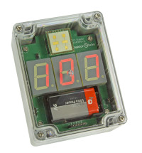
The circuit board is a double sided board with dimensions of 89 x 75 mm. The radar module and the seven segment displays are mounted on the top side and all the other components as well as the battery holder on the bottom side of the board. Most of the components are surface mount components. The dsPIC's package is 28-pin SSOP with a 0.65 mm pitch and it can be somewhat challenging to solder by hand. However, with a good soldering iron, even a modest microscope and some practice also the smallest components on the board can be soldered adequately. The dsPIC, which I used, is available also in DIP and SOIC packages but after getting some experience in soldering small SMD components I have started to prefer more compact components. The circuit board is mounted in a plastic box, which has a clear cover. Display can be clearly seen through the cover while the electronics are protected from ball hits for example. The radar was tested in a floorball training and it was noticed that it can detect a plastic ball with about 7 cm diameter from several meters distance. A car can be detected at distance of about 50 to 100 meters. I did not perform thorough validation of the speed measurement accuracy but at least the car speed measurements were in line with speeds given by my car's speedometer.Final thoughts
I am quite happy with the results of this project -- the final product is at least a nice toy and has potential in many other applications as well. The project turned out to be also very educative. This was the first time I used a digital signal controller. In previous projects I have used 8-bit microcontrollers and bigger processors like the ones used in Raspberry Pi and Beaglebone boards. It took some time to get the FFT processing, which is the core of the signal processing in this application, up and running. Explanatory examples and documentation provided by Microchips was great help in this task. Digital signal controller turned out to be reasonably efficient in this kind of signal processing task and it can be an interesting addition to my toolbox for future projects. If the radar module raised your interested it is not necessary to build a circuit board right away. I started experimenting with the module by connecting the IF outputs of the radar module to the sound card of my PC. In the PC I used the SDR# software which accepts the sound card signal as an input and has nice spectrum and spectrogram displays for inspecting the frequency content of the signal. With this kind of simple setup it is possible to get a good idea how the radar module operates and what kind of targets are detectable with it.References
- Gregory L. Charvat: The Future of Small Radar Technology, Circuit Cellar, April 2014.
- K-LC5 Radar Transceiver Data Sheet, RFbeam Microwave GmbH, https://www.rfbeam.ch/files/products/9/downloads/Datasheet_K-LC5.pdf.
- Software source code for dsPIC33EP128GP502
- Richard G. Lyons (ed.), Streamlining Digital Signal Processing, IEEE Press, 2007.
Mises à jour de l'auteur