
Conductivity Shield for Arduino Uno
This project describes a Conductivity Shield for Arduino Uno that allows you to accurately measure the conductivity of chemical solutions.
Conductivity is the ability of a material to transfer electrons. It is the opposite of the concept of resistivity which is well known to electricians. However, while we are used to address the topic of conductivity in the field of electronics, things get a little bit more complicated when we try to apply the concepts to chemical solutions such as salty water.
If I am addressing the topic here it is because measuring the conductivity of chemical solution is a pretty handy concept in lab or field operations. It can be used to monitor drinking water quality, find titrations end points, track reaction kinetics... All the applications usually rely on the fact that a solution conductivity is proportional to its salt concentration. The proportionality may vary from linear on small domains to more complex shapes that are best described by the Kohlrausch law on larger ranges. As an indication, the circuit presented here is able to track the concentration of sodium chloride (kitchen salt) in water from 1.5 mg/l to about 25 g/l with a typical deviation to linearity of 15%. This corresponds to the salinities of almost distilled water to sea water. Quite nice for a small circuit!
Conductivity measurement tools are readily available from chemical suppliers with price ranging from 300€ to more than 1,500€. Here, I wanted to make something affordable but accurate enough to be usable by the amateur scientist or by students to better understand and play with the concept of chemical conductivity. I therefore decided to build something around an Arduino UNO R3 with a LCD shield from Adafruit. A picture of the complete Arduino stack is shown in Figure 1 with the conductivity probe in a beaker on the right hand side of the image. You may also browse directly to the end of the post where Figure 11 shows a detailed picture of the conductivity shield presented here. All the Gerber files and BOM are included such that you can reproduce the circuit yourself.
To give an idea on how useful the circuit can be to undergrad students, Figure 2 shows a titration plot obtained with it in the lab. In the experiment, an acid of known concentration (oxalic acid) is slowly added to a solution of a base of unknown concentration (potassium carbonate here). As the acid (the titrant) is added to the solution, it neutralizes the base until all the base is consumed. After that point (called the equivalence point) the solution is becoming acidic because we keep adding acid to the solution and there is no more base to neutralize it. The experimental concept is to find the location of the equivalence point with precision such that we can infer the base concentration from the measurement. You have probably done this in high-school chemistry labs but with a coloured indicator that turned from pink to clear when the equivalence point was reached. The idea is exactly the same with the conductivity measurement except that it is much more precise. In Figure 2, the equivalence point is found by the intersection of two lines which represent the conductivity of excess base on the left and of excess acid on the right.
Now that the “why” is better understood, let us discuss the “how”!
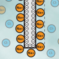
If you have ever tried to plug your ohm-meter to a glass of water you know that it does not work. Instead, you will measure a constantly changing voltage. This is because chemical solutions do not transfer electrons like a copper wire would do. Instead, the electrons flow to the electrodes and get stuck on the walls, just as they would do in a capacitor. This is represented for a solution of sodium chloride (Na+ and Cl- ions) in Figure 3. One of the electrode charges negatively and calls in for positive sodium (Na+) ions while the other charges positively and calls in for negative chloride (Cl-) ions. Note that at some point the layer of ions formed on the electrodes will repel the other ions and some steady state is quickly reached. The situation is exactly similar to that of a capacitor and we may actually find a good approximation of the impedance of the system by using the capacitor estimations laws with a thickness equal to about the width of the ions layer that is on the order of 0.1-1 nm. Typical capacitances are therefore on the range of 10-100 µF depending on the electrode construction. This is known as the Helmholtz outer layer theory and more advanced models exist but it is already enough to get a basic understanding on what is going on there.
This explains why you cannot use a common ohm-meter that is based on a DC voltage. Instead, we must use AC voltage. However, at high frequencies the two electrodes also form a capacitor and we start losing current by a by-pass effect. The ideal operation frequency will depend on the electrode construction and the salinity of the solution. Figure 4 shows the experimental transfer function obtained at different NaCl concentration. More concentrated solutions have an apex located towards the lower frequencies and it is clear that we cannot use frequencies above 10 kHz here because of the bypass effect that will strongly affect the measurement. As a compromise, I decided to build the circuit excitation frequency at roughly 7 kHz such that I could work with a large range of concentrations.
The electrode is a big part of the measurement tool and working with a bad electrode can ruin your result. Whereas commercial probes are made from expensive platinized platinum I decided to make one from a cheap PCB layout with gold plating. The electrode is shown in Figure 5. The two wires were soldered at the bottom of the electrode and insulated using an epoxy adhesive (Scotchweld 2216). Surprisingly, I got really good results with these electrodes and they even survived in bleach! I have included the Gerber files for the electrode as well so that you can easily reproduce it. The only recommendation that I could make is to clean the probe with distilled water after usage to prevent oxidation.
All of that discussion was true at low excitation voltages but as we increase the voltage, sometimes as low as 100 mVolts, the electrodes may become reactive enough to actually achieve transfer of electrons from/to the solution. When this occurs, the actual composition of the solution changes in a reaction known as electrolysis. In the case of sodium chloride solution, toxic and explosive chlorine and hydrogen gas will be produced. We must therefore limit our circuit to low excitation voltage, 50 mVolts maximum to be safe. The good news is that the currents involved will therefore be relatively low and we can work with classical operational amplifiers such as the TL074 to provide the excitation frequency and perform the current measurement. It is important to understand that the current measured from this electron flow does not represent the solution conductivity but only the speed of the electrolysis process which is completely irrelevant to us.
The overall measurement concept is shown in Figure 6. A 7 kHz sine wave oscillator of ~50 mVolts amplitude is fed to a probe put in the solution to measure and the other end of the probe connected to a current to voltage converter with selectable gain. The output voltage is then fed into a RMS converter to get the amplitude of the current and sent to the Arduino analog input pin. A copy of the 7 kHz source is also sent to a RMS converter to act as a reference voltage for the Arduino. This way, any fluctuations in the oscillation amplitudes will be compensated and we will measure directly the conductivity of the solution. Finally, and to cope with more concentrated solution, I added a 1:10 divider switch to artificially reduce the input wave amplitude to about 5 mVolts. In practice, this does work but the results tend to be noisier.
Let us now check how each part of the circuit was implemented.
The source with the divider switch is shown in Figure 7. It is based on a 5 stages RC oscillator (R1-4, R9 and C1-C5) with feedback gain made from resistors R5 and R6. RV1 trimmer allows tuning the output amplitude to about 50 mVolts RMS and R18/R19 do the 1:10 reduction when the analog switch MAX4605 is enabled through the “high conductivity enable” pin. U1:D acts as a follower to deliver the required current to the probe.
The sine wave reference is then fed to the RMS circuit of Figure 8. It consists of a first inverting amplifier U5:A of tuneable gain (through trimmer RV2) and full-wave rectifier made from U5:B and U5:C before entering in the low-pass filter of U5:D. The low-pass cut-off frequency is fixed by resistor R22-23 and capacitors C10-C11. They are non-critical and so standard components can be used. We only need them to remove the carrier frequency at 7 kHz. On the other hand, it is important to use matched resistors for R24-R28 because they may distort the shape of the rectified signal and produce RMS reading errors. I recommend using at least 1% resistors and, if possible, 0.1% one or to match them from a larger batch prior to soldering. During experimentation, I noticed that the gain of RV2+R20/R29 was too high and I would now recommend increasing R29 to probably 10 kΩ or more.
The second electrode of the probe is connected to the current sensing circuit shown in Figure 9. It is made of a current-to-voltage converter with selectable gain and of a RMS converter similar to the one of Figure 8 (do not forget to match resistors R34-R38 therefore!). The current-to-voltage converter have gains of 1,800 V/A, 18,000 V/A and 180,000 V/A that can be activated using the analog switches MAX4605 through the pins “RES1-3 ENABLE”. This part of the circuit is not optimal and I had some issues with it. While it is working, a better idea would have been to add a final ~1.8 MΩ resistor in parallel to extend the range or to use a DG408 1:8 multiplexer circuit to have more gains with 1:3 ratios instead of the current 1:10 ratios that sometimes make you lose resolution when switching the conductivity ranges. If you plan to revise the circuit, I would recommend 1 kΩ, 3.3 kΩ, 10 kΩ, 33 kΩ, 100 kΩ, 330 kΩ, 1 MΩ and 3.3 MΩ resistors for the gains instead. The high conductivity switch made with the last MAX4605 could then be replaced by a DG469 if not discarded at all.
Finally, a TC962 DC-to-DC inverter is used to produce the split supply for the op amps using the 12 Volts input from the Arduino. Although its clock frequency is close to the source frequency we are using (7 kHz) I did not notice noise coupling into the signal and so the circuit can be kept as it.
Because of the relatively large amount of components involved, the circuit was implemented in SMT to keep the size to that of an Arduino UNO board. The circuit is however not particularly hard to solder as standard 1206 components were used. Still, I recommend to use a stencil to correctly apply the tin to the board before adding the components. The circuit with its probe is shown in Figure 11. Please note the insertion position of the probe in the socket header.
When testing the circuit, plug it on the Arduino shield with a 12 Volts power supply and adjust the trimmer RV1 until the probe output “probe+” reaches 50 mVolts RMS. Then, adjust trimmer RV2 such that the reference voltage goes above 1.5 Volts. Be careful not to go too high because you will get a messed-up/distorted voltage. Once this is done, just plug-in the LCD shield and the probe!
For your first tests on the field just take a glass of tap water and put the probe into it. Then, slowly add kitchen salt to the water in very small amounts and you should see the conductivity changing (you may have to swirl the glass a little bit to homogenise the solution). After that, you can try whatever you want: water from a river, a lake, rain water… Remember to clean the probe with tap water to extend its life if you plan to use concentrated salt solutions such as sea water.
If you would like to go “pro” you can also order standardized conductivity solutions from chemical suppliers such as 5,000 mS/cm solutions to calibrate the conductometer. Begin first by measuring the conductivity of the standard solution with the circuit and then modify the Arduino code. At the very beginning of the file there is a variable called “g_fCalibration”. If this field is set to zero the program will display raw units but if you set this field to the value outputted with a 5,000 mS/cm solution it will automatically convert the reading to a value in mS/cm. Do not forget that conductivity is temperature dependant so it is possible that your measurement will change depending on the ambient temperature!
* This article is an extended version of a circuit presented on my website http://www.thepulsar.be in summer 2016.
If I am addressing the topic here it is because measuring the conductivity of chemical solution is a pretty handy concept in lab or field operations. It can be used to monitor drinking water quality, find titrations end points, track reaction kinetics... All the applications usually rely on the fact that a solution conductivity is proportional to its salt concentration. The proportionality may vary from linear on small domains to more complex shapes that are best described by the Kohlrausch law on larger ranges. As an indication, the circuit presented here is able to track the concentration of sodium chloride (kitchen salt) in water from 1.5 mg/l to about 25 g/l with a typical deviation to linearity of 15%. This corresponds to the salinities of almost distilled water to sea water. Quite nice for a small circuit!
Conductivity measurement tools are readily available from chemical suppliers with price ranging from 300€ to more than 1,500€. Here, I wanted to make something affordable but accurate enough to be usable by the amateur scientist or by students to better understand and play with the concept of chemical conductivity. I therefore decided to build something around an Arduino UNO R3 with a LCD shield from Adafruit. A picture of the complete Arduino stack is shown in Figure 1 with the conductivity probe in a beaker on the right hand side of the image. You may also browse directly to the end of the post where Figure 11 shows a detailed picture of the conductivity shield presented here. All the Gerber files and BOM are included such that you can reproduce the circuit yourself.
To give an idea on how useful the circuit can be to undergrad students, Figure 2 shows a titration plot obtained with it in the lab. In the experiment, an acid of known concentration (oxalic acid) is slowly added to a solution of a base of unknown concentration (potassium carbonate here). As the acid (the titrant) is added to the solution, it neutralizes the base until all the base is consumed. After that point (called the equivalence point) the solution is becoming acidic because we keep adding acid to the solution and there is no more base to neutralize it. The experimental concept is to find the location of the equivalence point with precision such that we can infer the base concentration from the measurement. You have probably done this in high-school chemistry labs but with a coloured indicator that turned from pink to clear when the equivalence point was reached. The idea is exactly the same with the conductivity measurement except that it is much more precise. In Figure 2, the equivalence point is found by the intersection of two lines which represent the conductivity of excess base on the left and of excess acid on the right.
Now that the “why” is better understood, let us discuss the “how”!
If you have ever tried to plug your ohm-meter to a glass of water you know that it does not work. Instead, you will measure a constantly changing voltage. This is because chemical solutions do not transfer electrons like a copper wire would do. Instead, the electrons flow to the electrodes and get stuck on the walls, just as they would do in a capacitor. This is represented for a solution of sodium chloride (Na+ and Cl- ions) in Figure 3. One of the electrode charges negatively and calls in for positive sodium (Na+) ions while the other charges positively and calls in for negative chloride (Cl-) ions. Note that at some point the layer of ions formed on the electrodes will repel the other ions and some steady state is quickly reached. The situation is exactly similar to that of a capacitor and we may actually find a good approximation of the impedance of the system by using the capacitor estimations laws with a thickness equal to about the width of the ions layer that is on the order of 0.1-1 nm. Typical capacitances are therefore on the range of 10-100 µF depending on the electrode construction. This is known as the Helmholtz outer layer theory and more advanced models exist but it is already enough to get a basic understanding on what is going on there.
This explains why you cannot use a common ohm-meter that is based on a DC voltage. Instead, we must use AC voltage. However, at high frequencies the two electrodes also form a capacitor and we start losing current by a by-pass effect. The ideal operation frequency will depend on the electrode construction and the salinity of the solution. Figure 4 shows the experimental transfer function obtained at different NaCl concentration. More concentrated solutions have an apex located towards the lower frequencies and it is clear that we cannot use frequencies above 10 kHz here because of the bypass effect that will strongly affect the measurement. As a compromise, I decided to build the circuit excitation frequency at roughly 7 kHz such that I could work with a large range of concentrations.
The electrode is a big part of the measurement tool and working with a bad electrode can ruin your result. Whereas commercial probes are made from expensive platinized platinum I decided to make one from a cheap PCB layout with gold plating. The electrode is shown in Figure 5. The two wires were soldered at the bottom of the electrode and insulated using an epoxy adhesive (Scotchweld 2216). Surprisingly, I got really good results with these electrodes and they even survived in bleach! I have included the Gerber files for the electrode as well so that you can easily reproduce it. The only recommendation that I could make is to clean the probe with distilled water after usage to prevent oxidation.
All of that discussion was true at low excitation voltages but as we increase the voltage, sometimes as low as 100 mVolts, the electrodes may become reactive enough to actually achieve transfer of electrons from/to the solution. When this occurs, the actual composition of the solution changes in a reaction known as electrolysis. In the case of sodium chloride solution, toxic and explosive chlorine and hydrogen gas will be produced. We must therefore limit our circuit to low excitation voltage, 50 mVolts maximum to be safe. The good news is that the currents involved will therefore be relatively low and we can work with classical operational amplifiers such as the TL074 to provide the excitation frequency and perform the current measurement. It is important to understand that the current measured from this electron flow does not represent the solution conductivity but only the speed of the electrolysis process which is completely irrelevant to us.
The overall measurement concept is shown in Figure 6. A 7 kHz sine wave oscillator of ~50 mVolts amplitude is fed to a probe put in the solution to measure and the other end of the probe connected to a current to voltage converter with selectable gain. The output voltage is then fed into a RMS converter to get the amplitude of the current and sent to the Arduino analog input pin. A copy of the 7 kHz source is also sent to a RMS converter to act as a reference voltage for the Arduino. This way, any fluctuations in the oscillation amplitudes will be compensated and we will measure directly the conductivity of the solution. Finally, and to cope with more concentrated solution, I added a 1:10 divider switch to artificially reduce the input wave amplitude to about 5 mVolts. In practice, this does work but the results tend to be noisier.
Let us now check how each part of the circuit was implemented.
The source with the divider switch is shown in Figure 7. It is based on a 5 stages RC oscillator (R1-4, R9 and C1-C5) with feedback gain made from resistors R5 and R6. RV1 trimmer allows tuning the output amplitude to about 50 mVolts RMS and R18/R19 do the 1:10 reduction when the analog switch MAX4605 is enabled through the “high conductivity enable” pin. U1:D acts as a follower to deliver the required current to the probe.
The sine wave reference is then fed to the RMS circuit of Figure 8. It consists of a first inverting amplifier U5:A of tuneable gain (through trimmer RV2) and full-wave rectifier made from U5:B and U5:C before entering in the low-pass filter of U5:D. The low-pass cut-off frequency is fixed by resistor R22-23 and capacitors C10-C11. They are non-critical and so standard components can be used. We only need them to remove the carrier frequency at 7 kHz. On the other hand, it is important to use matched resistors for R24-R28 because they may distort the shape of the rectified signal and produce RMS reading errors. I recommend using at least 1% resistors and, if possible, 0.1% one or to match them from a larger batch prior to soldering. During experimentation, I noticed that the gain of RV2+R20/R29 was too high and I would now recommend increasing R29 to probably 10 kΩ or more.
The second electrode of the probe is connected to the current sensing circuit shown in Figure 9. It is made of a current-to-voltage converter with selectable gain and of a RMS converter similar to the one of Figure 8 (do not forget to match resistors R34-R38 therefore!). The current-to-voltage converter have gains of 1,800 V/A, 18,000 V/A and 180,000 V/A that can be activated using the analog switches MAX4605 through the pins “RES1-3 ENABLE”. This part of the circuit is not optimal and I had some issues with it. While it is working, a better idea would have been to add a final ~1.8 MΩ resistor in parallel to extend the range or to use a DG408 1:8 multiplexer circuit to have more gains with 1:3 ratios instead of the current 1:10 ratios that sometimes make you lose resolution when switching the conductivity ranges. If you plan to revise the circuit, I would recommend 1 kΩ, 3.3 kΩ, 10 kΩ, 33 kΩ, 100 kΩ, 330 kΩ, 1 MΩ and 3.3 MΩ resistors for the gains instead. The high conductivity switch made with the last MAX4605 could then be replaced by a DG469 if not discarded at all.
Finally, a TC962 DC-to-DC inverter is used to produce the split supply for the op amps using the 12 Volts input from the Arduino. Although its clock frequency is close to the source frequency we are using (7 kHz) I did not notice noise coupling into the signal and so the circuit can be kept as it.
Because of the relatively large amount of components involved, the circuit was implemented in SMT to keep the size to that of an Arduino UNO board. The circuit is however not particularly hard to solder as standard 1206 components were used. Still, I recommend to use a stencil to correctly apply the tin to the board before adding the components. The circuit with its probe is shown in Figure 11. Please note the insertion position of the probe in the socket header.
When testing the circuit, plug it on the Arduino shield with a 12 Volts power supply and adjust the trimmer RV1 until the probe output “probe+” reaches 50 mVolts RMS. Then, adjust trimmer RV2 such that the reference voltage goes above 1.5 Volts. Be careful not to go too high because you will get a messed-up/distorted voltage. Once this is done, just plug-in the LCD shield and the probe!
For your first tests on the field just take a glass of tap water and put the probe into it. Then, slowly add kitchen salt to the water in very small amounts and you should see the conductivity changing (you may have to swirl the glass a little bit to homogenise the solution). After that, you can try whatever you want: water from a river, a lake, rain water… Remember to clean the probe with tap water to extend its life if you plan to use concentrated salt solutions such as sea water.
If you would like to go “pro” you can also order standardized conductivity solutions from chemical suppliers such as 5,000 mS/cm solutions to calibrate the conductometer. Begin first by measuring the conductivity of the standard solution with the circuit and then modify the Arduino code. At the very beginning of the file there is a variable called “g_fCalibration”. If this field is set to zero the program will display raw units but if you set this field to the value outputted with a 5,000 mS/cm solution it will automatically convert the reading to a value in mS/cm. Do not forget that conductivity is temperature dependant so it is possible that your measurement will change depending on the ambient temperature!
* This article is an extended version of a circuit presented on my website http://www.thepulsar.be in summer 2016.
Want to build a project?
Bring your design to life with the Elektor PCB Service, powered by Eurocircuits. Upload the project files and order professionally manufactured PCBs or assembled boards through a proven European production platform.
Supporting KiCad, Eagle, Gerber, and ODB++ formats, the service is suitable for everything from prototypes and validation builds to series production and volume manufacturing.
Made in Europe. Fast. Reliable. Professional.
Discussion (2 commentaire(s))